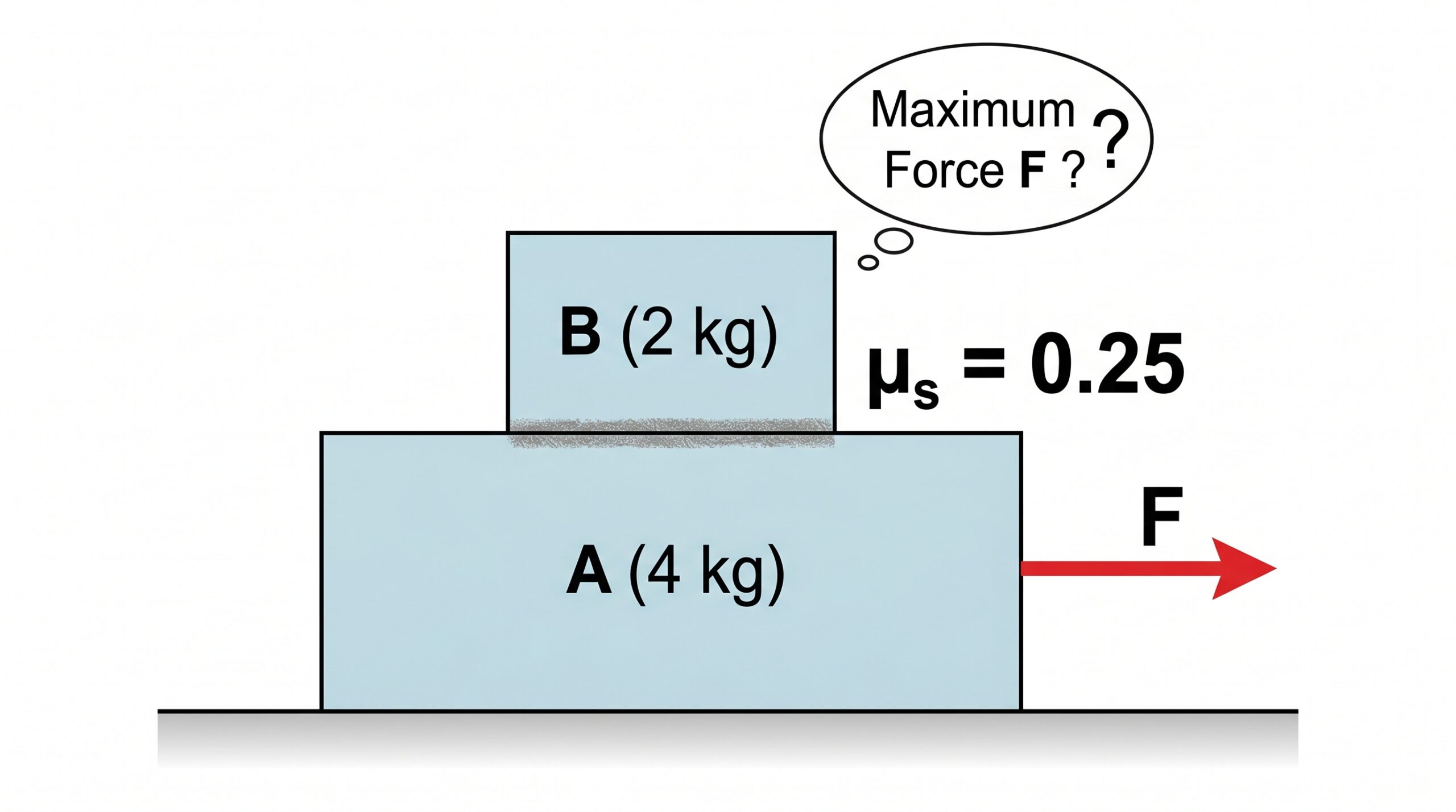
Maximum Force such that both blocks move together

Maximum Force such that both blocks move together

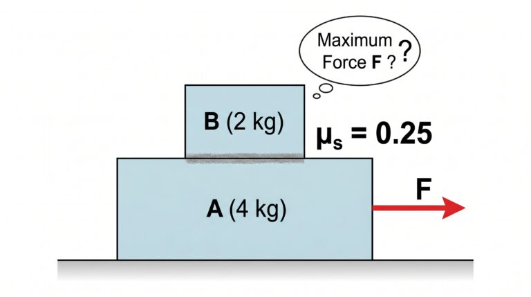
A block A (mass 4 kg) is placed on a smooth horizontal surface. Another block B (mass 2 kg) is placed on top of A. A horizontal force F is applied to block A as shown. The coefficient of static friction between the two blocks is μ = 0.25. Find the maximum value of force F such that both blocks move together without slipping.

Maximum Force such that both blocks move together

Complete Video Solution below

Maximum Force such that both blocks move together Without Slipping: Understanding the Real Physics

One of the most common friction problems in JEE Main, JEE Advanced, and NEET involves two blocks placed one above the other. A horizontal force is applied to the lower block, and students are asked to find the maximum force that can be applied so that both blocks move together without slipping.

At first glance, this may look like a standard formula-based problem. However, the real value of this question lies in the concepts it teaches.

In fact, many students solve such problems mechanically without understanding the actual role of friction. As a result, they often make mistakes when the problem is slightly modified.

Before jumping to equations, let us first understand the physics behind this situation.

The First Question: How Does the Upper Block Move?

Suppose a force is applied to the lower block.

The lower block is directly connected to the external force, so it is obvious why it starts moving.

But what about the upper block?

No force is directly applied to it.

So why should it move at all?

This is the most important question in the entire problem.

Before writing equations, always ask yourself:

What is the force responsible for accelerating the upper block?

Once you answer this question, the entire problem becomes much easier.

Many students immediately start looking for formulas.

A better approach is to first understand the physics.

Do not start with formulas. Start with physics.

The Hero of the Story: Static Friction

The upper block moves because of static friction.

Many students think friction only opposes motion.

This is not entirely true.

A more accurate statement is:

Friction opposes relative motion or the tendency of relative motion between two surfaces.

In this problem, the lower block tries to move forward. If there were no friction, the lower block would slide out from beneath the upper block.

Static friction prevents this from happening.

It pulls the upper block forward and allows both blocks to move together.

Therefore, static friction is not acting as an enemy here.

It is actually helping the upper block move.

This is a very important idea that students should remember.

Static Friction Is Smarter Than Most Students Think

Many students believe that static friction is always equal to μN.

This is one of the most common misconceptions in mechanics.

Static friction is not a fixed force.

It adjusts itself according to the requirement of the situation.

If a small friction force is needed, static friction provides a small force.

If a larger friction force is needed, static friction increases its value.

However, it cannot increase forever.

There is a maximum limit beyond which static friction cannot go.

As long as the required friction remains below this limit, the blocks continue to move together.

The moment the required friction exceeds this limit, slipping begins.

Understanding this single idea can solve a large number of friction problems.

Why Friction Direction Confuses Students

One of the most common mistakes in friction problems is assuming the wrong direction of friction.

Students often memorize rules instead of thinking physically.

The correct approach is simple.

Ask yourself:

If friction were absent, what would happen?

Without friction, the lower block would move forward while the upper block would tend to stay where it is because of inertia.

Therefore, relative to the lower block, the upper block would appear to move backward.

Static friction opposes this tendency.

As a result, friction acts forward on the upper block.

According to Newton’s Third Law, an equal and opposite friction force acts backward on the lower block.

The direction becomes obvious once you understand the physical situation.

A Common Mistake Students Make

Many students immediately draw friction opposite to the motion of the object.

This shortcut often creates confusion.

Remember:

Friction does not oppose motion. Friction opposes relative motion.
This small distinction can completely change the solution.

Whenever you are confused about friction direction, imagine the situation without friction.

The correct direction usually becomes obvious.

A small mistake here can spoil the entire problem.

As teachers often say:

A small mistake in friction direction can make the entire solution go wrong.

Moving Together Means No Slipping

The statement “both blocks move together” is extremely important.

It tells us that there is no relative motion between the two blocks.

Since there is no slipping, kinetic friction does not come into the picture.

Only static friction is acting.

Many students immediately use friction formulas without first identifying the type of friction involved.

This is dangerous.

Always determine whether slipping is occurring or not before choosing the friction model.

As long as the two blocks move together, static friction is responsible for maintaining the common motion.
Can Static Friction Do the Job?

Now we come to the central idea of the problem.

The upper block needs a certain force to accelerate along with the lower block.

That force is supplied by static friction.

However, static friction is not unlimited.

It has a maximum possible value.

As the applied force on the system increases, the acceleration of the system increases.

A larger acceleration means the upper block requires a larger friction force.

Initially, static friction can easily provide the required force.

But as the applied force keeps increasing, a stage is reached where the required friction becomes equal to the maximum friction available.

This is the limiting situation.

At this point, static friction is working at its highest possible value.

This condition determines the maximum force that can be applied while keeping both blocks together.

What Happens Beyond This Limit?

Suppose we increase the applied force even further.

Now the upper block requires more friction than static friction can provide.

But friction cannot exceed its maximum limit.

As a result, static friction fails to maintain common motion.
The upper block can no longer keep up with the lower block.

Relative motion begins.

Slipping starts.

The moment slipping starts, static friction disappears and kinetic friction takes over.

This is why the problem asks for the maximum force.

It is asking for the boundary between two situations:

  1. Both blocks move together.

  2. The upper block starts slipping.

Understanding this boundary is much more important than memorizing any formula.

Why This Problem Is More Important Than It Looks

At first glance, this appears to be a simple two-block friction problem.

However, the ideas used here appear again and again in mechanics.

The same concepts are used in:

  • Friction problems

  • Wedge problems

  • Pulley systems

  • Circular motion with friction

  • Advanced Newton’s Laws questions

The goal is not to remember an answer.

The goal is to understand how forces interact and how friction helps maintain common motion.
Once you understand the physics behind this question, many seemingly difficult problems become much easier.

Physics Is About Understanding, Not Memorization

Many students search for shortcuts and formulas.

However, formulas are only the final result of physical reasoning.

If you understand the role of friction, the direction of friction, and the condition for slipping, you can derive the result whenever required.

That is the real goal of learning physics.

The two-block friction problem teaches us something far more valuable than a numerical answer.

It teaches us how static friction helps two surfaces maintain common motion and how slipping begins when friction reaches its limit.

Once this concept becomes clear, many friction problems become surprisingly simple.

Remember:

Do not start with formulas. Start with physics.

When the physics is clear, the mathematics becomes easy.

Final Solution

Given:
m_A\;=\;4\;kg

m_B=2kg
\mu_s=0.25
Maximum static friction:

f_{max\;=\;\mu_s\;m_B\;g}

System acceleration at limiting condition:

a_{max\;=\;\mu_s\;\;g}
a_{max\;=\;0.25\times\;\;10}
a_{max}=\;2.5\;m/s^2

For the complete system:

Fmax=(mA+mB)amaxF_{max}=(m_A+m_B)a_{max} Fmax=6×2.5=15 NF_{max}=6\times2.5=15\,N

Answer: Fmax=15NF_{max}=15N

Author: Deep Aman Sir

Founder, PCM TUTORIALS | Physics Faculty for JEE, NEET & CBSE

Online Physics Classes

              Online Physics Classes by Mr. Deep Aman 

Welcome to the Online Physics Classes program by PCM TUTORIALS.
These classes are specially designed for students preparing for JEE Main, JEE Advanced, NEET, and CBSE Board examinations.

Physics is taught with a strong focus on:

  • Conceptual clarity
  • Advanced problem solving
  • Visualization and derivations
  • Numerical applications
  • Real understanding of Physics

Classes are conducted live by Mr. Deep Aman, who has been teaching competitive Physics since 2015. 

Mr. Deep Aman is the founder of PCM TUTORIALS. With over 10 years of experience in teaching Physics in offline classroom settings, he has now transitioned to the online platform to expand his reach and help a wider range of students.

His teaching approach focuses on deep conceptual clarity, problem-solving skills, and simplifying complex Physics topics for JEE, NEET, and board aspirants through a structured digital learning system.

Live Online Physics  Classes on Zoom

Interactive live classes are conducted regularly on Zoom where students can:

  • Learn concepts step-by-step
  • Ask doubts during class
  • Practice numerical problems
  • Understand derivations deeply
  • Improve problem-solving speed and accuracy
    •  

Features of Our Online Physics Classes

    • Live Zoom Sessions
    • Doubt Discussion
    • Topic-wise Assignments
    • Practice Questions
    • Conceptual Learning
    • Regular Tests
    • Personal Guidance


Who Can Join?

  • Class 11 Students
  • Class 12 Students
  • JEE Aspirants
  • NEET Aspirants
  • CBSE Students


Small Batch Personalized Learning

Each batch is either personalized or consists of a group of fewer than 5 students to ensure individual attention, better interaction, and strong conceptual understanding.

Know Your Tutor

To know your teacher, teaching methodology, dedication towards Physics, and conceptual style of teaching, visit our YouTube channel:

Deep Aman Online Physics

PhysicsEduMedia

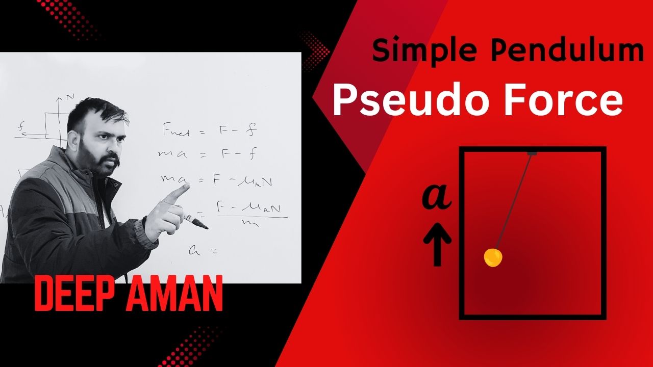
Pseudo Force

Pseudo Force

Pseudo Force: Understanding the “Fictitious” Force of Non-Inertial Frames

Physics is full of concepts that seem counterintuitive at first but become fascinating once you dive deeper. One such idea is the pseudo force (sometimes called fictitious force).

Whenever you sit in a bus that suddenly accelerates or take a sharp turn in a car, you feel as if some mysterious force is acting on you, pushing you backward or sideways. But in reality, there is no such physical agent pushing you. That’s the world of pseudo force — a force that appears only when we observe motion from a non-inertial reference frame.

This article will explore pseudo force in detail — its definition, origin, mathematical expression, examples, and applications. By the end, you’ll understand why pseudo forces are not “real” in the strict sense, yet are extremely useful in solving problems of mechanics.


1. Reference Frames: The Foundation

Before talking about pseudo force, we need to revisit the concept of reference frames.

  • Reference Frame: A coordinate system from which we observe and measure the motion of objects.

  • Inertial Frame: A frame of reference in which Newton’s laws of motion hold true without modification. Typically, a frame at rest or moving with constant velocity relative to the “fixed stars” is considered inertial.
  • Non-Inertial Frame: A frame that is accelerating or rotating relative to an inertial frame. In such frames, Newton’s laws do not appear to hold unless we introduce additional forces — the pseudo forces.

Example:

  1. Standing on the ground (which we approximate as an inertial frame for most problems), you see a ball falling vertically under gravity.

  2. Sitting in an accelerating car (a non-inertial frame), the same ball seems to move backward, even though no physical backward force is acting on it.


2. What is a Pseudo Force?

Definition:
A pseudo force is an apparent force that arises when we describe motion from a non-inertial frame. It has no physical interaction or agent behind it. Instead, it is introduced mathematically to make Newton’s second law applicable inside a non-inertial frame.

Key Points:

  • It is not a “real” force — it doesn’t arise due to any physical contact or field.

  • It is proportional to the mass of the object.

  • It always acts opposite to the acceleration of the non-inertial frame with respect to the inertial frame.


3. Mathematical Expression of Pseudo Force

Suppose we have:

  • An inertial frame SS.

  • A non-inertial frame S’S’, accelerating with acceleration a⃗0\vec{a}_0 relative to SS.

  • An object of mass mm.

In inertial frame SS:

ma⃗=∑F⃗realm\vec{a} = \sum \vec{F}_{\text{real}}

But in non-inertial frame S’S’:
The acceleration of the object relative to S’S’ is different, so Newton’s law does not balance unless we introduce a fictitious force:

ma⃗′=∑F⃗real+F⃗pseudom\vec{a}’ = \sum \vec{F}_{\text{real}} + \vec{F}_{\text{pseudo}}

Where,

F⃗pseudo=−ma⃗0\vec{F}_{\text{pseudo}} = -m\vec{a}_0

Thus, the pseudo force is directly proportional to the mass of the body and opposite to the acceleration of the non-inertial frame.


4. Everyday Examples of Pseudo Force

(i) The Bus Ride

  • When a bus suddenly accelerates forward, passengers feel a backward push.

  • From the ground (inertial frame), passengers tend to remain at rest due to inertia.

  • From the bus frame (non-inertial), it looks as if a backward force is pushing them. That is the pseudo force.

(ii) Elevator Problems

  • In a downward accelerating lift, a person feels lighter.

  • In an upward accelerating lift, the person feels heavier.

  • The apparent weight is explained by introducing pseudo force equal to −ma0 -ma_0, where a0a_0 is the acceleration of the lift.

(iii) Rotating Reference Frames (Centrifugal Force)

  • When you take a sharp turn in a car, you feel “thrown” outward.

  • From the inertial frame, you are simply trying to maintain a straight-line path, but the car is turning beneath you.

  • From the rotating (car’s) frame, an outward pseudo force called the centrifugal force appears.

(iv) Coriolis Force

  • A special pseudo force observed in rotating frames, responsible for large-scale effects like trade winds, cyclones, and ocean currents on Earth.


5. Pseudo Force vs Real Force

Feature Real Force Pseudo Force
Origin Arises from physical interaction (contact, field, gravity, electromagnetism, etc.) Arises due to acceleration of reference frame
Agent Always has a physical source No physical agent
Newton’s Laws Can be explained directly by Newton’s second law Introduced to make Newton’s laws valid in non-inertial frames
Example Gravitational force, tension, friction Backward push in an accelerating bus, centrifugal force

6. Types of Pseudo Forces (Required for JEE/NEET level)

  1. Linear Acceleration Pseudo Force: Appears when the frame is linearly accelerating.

    • Expression: F⃗pseudo=−ma⃗0\vec{F}_{\text{pseudo}}=-m\vec{a}_0.

  2. Centrifugal Force: Appears in rotating frames, directed radially outward.

    • Expression: Fc=mω2rF_c = m\omega^2 r.


7. Pseudo Force in Elevators – A Classic Example

Let’s derive the apparent weight in a lift:

  • Actual weight = mgmg.

  • Lift acceleration = aa.

In the elevator’s frame:

Apparent weight=N=mg−Fpseudo\text{Apparent weight} = N = mg – F_{\text{pseudo}}

Where pseudo force = −ma -ma.

So,

  • If lift accelerates upward (a>0a>0):
    N=mg+maN = mg + ma. → You feel heavier.

  • If lift accelerates downward (a>0a>0):
    N=mg−maN = mg – ma. → You feel lighter.

  • If a=ga=g (free fall): N=0N=0. → Weightlessness.


8. Pseudo Force in Rotating Frames – Centrifugal and Coriolis

When a body is in a rotating frame (like a rotating merry-go-round), it seems to be “thrown” outward.

  • From inertial frame: The body tries to move tangentially (straight line).

  • From rotating frame: An outward pseudo force F=mω2rF=m\omega^2 r is introduced to explain the tendency.


9. Applications of Pseudo Forces

  1. Engineering and Design:

    • Designing elevators, centrifuges, rotating machines.

    • Vehicle safety, roller-coaster rides, airplane maneuvers.

  2. Meteorology:

    • Coriolis force explains trade winds, cyclones, jet streams.

  3. Space Science:

    • Artificial gravity in rotating space stations uses centrifugal pseudo force.

  4. Daily Life:

    • Balancing in buses or trains, predicting motion while turning.

  5. Education:

    • Helps students reconcile Newton’s laws with real-life observations in accelerating systems.


10. Common Misconceptions

  • Pseudo forces are imaginary, so they are useless.
    Wrong! They are extremely useful tools to simplify analysis in non-inertial frames.

  • Centrifugal force pushes objects outward.
    In reality, no outward force exists in the inertial frame. It is the inertia of motion that makes objects resist circular motion.
  • Pseudo forces are optional.
    If you are working in a non-inertial frame, you must include them to apply Newton’s laws consistently.


11. Visualizing Pseudo Forces

If you are writing this for a blog, here are diagrams you can add (describe in captions):

  1. Passenger being thrown backward in an accelerating bus.

  2. Elevator free-fall with zero apparent weight.

  3. Centrifugal force on a ball tied to a rotating string.

  4. Coriolis effect deflection on Earth.

These visuals help readers connect theory with experience.


12. Pseudo Force and General Relativity – A Deeper Note

Interestingly, pseudo forces give a glimpse into Einstein’s general relativity. Gravity itself can be thought of as a pseudo force that arises because we observe motion from a non-inertial frame of curved spacetime.

In Einstein’s view:

  • Objects in free fall are actually in inertial motion (no real force).

  • Observers standing on Earth feel a downward “gravitational force” only because the Earth is accelerating upward relative to free-falling objects.

Thus, pseudo force in Newtonian mechanics acts as a stepping stone to understanding modern physics.


13. Summary

  • Pseudo force arises in non-inertial frames.

  • Formula: F⃗pseudo=−ma⃗0\vec{F}_{\text{pseudo}} = -m\vec{a}_0.

  • Examples include the backward push in an accelerating bus, elevator apparent weight, centrifugal and Coriolis forces.

  • They are not “real” but are extremely useful in calculations.

  • They connect classical mechanics to deeper ideas in relativity.


14. Conclusion

Next time you feel pushed backward in a speeding bus, remember — it’s not a mysterious hidden hand but your own inertia seen from a non-inertial frame. The pseudo force is a clever tool invented by physicists to keep Newton’s laws working consistently even in accelerating systems.

Understanding pseudo force enriches our grasp of dynamics, helps us appreciate everyday experiences, and lays a foundation for advanced physic

List of Important Physics derivations for Board Examinations (2024-25)

List of Important Physics derivations for Board Examinations (2024-25)

CBSE: Class-XII

Important Physics derivations for Board Examinations

Chapter 7 – Alternating Current (AC)


1.Using phasor diagram, derive an expression for voltage, current and impedance in LCR series circuit connected with alternating source of emf ɛ=sin(ωt + ф) . Also, deduce power factor of circuit  

2.In a series LCR circuit connected to an a.c. source of voltage, ɛ= sinωt.  Use phasor diagram to derive an expression for the current in the circuit. Hence, obtain the expression for the power dissipated in the circuit. Show that power dissipated at resonance is maximum.

3.A series LCR circuit is connected to an ac source. Using the phasor diagram, derive the expression for the impedance of the circuit. Plot a graph to show the variation of current with frequency of the source, explaining the nature of its variation.
4.Derive an expression for average power consumed/dissipated in series LCR circuit connected to alternating source in which the phase difference between volage(emf) and current is ф.

5.Define mean/average value of alternating current and show that the average current for half cycle of A.C. is    , where Io is peak current value.

6.Define mean/average value of alternating current and show that the average current for full cycle of A.C. is  zero  , where Io is peak current value.

7.Define r.m.s. value of alternating current and show that the r.m.s. value of current for half cycle of A.C. is    , where Io is peak current value.

8.Define r.m.s. value of alternating current and show that the r.m.s. value of current for full cycle of A.C. is    , where Io is peak current value.

9.Show that average power dissipated in pure inductor is zero when it is connected to A.C. supply . [2 Marks]

10.Show that average power dissipated in pure capacitor is zero when it is connected to A.C. supply . [2 Marks]

9.Show that average power dissipated in pure inductor is zero when it is connected to A.C. supply . [3 Marks]

10.Show that average power dissipated in pure capacitor is zero when it is connected to A.C. supply . [3 Marks]

11.Show that current leads voltage (emf) by phase angle  in pure capacitive circuit with capacitance C when it is connected to A.C. source. [3 Marks]

12.Show that the voltage (emf) leads current by phase angle  in pure inductive circuit with capacitance C when it is connected to A.C. source. [3 Marks]

Important Physics derivations for Board Examinations

Chapter 6 – Electromagnetic Induction (EMI)6

1.A conducting rod of length ℓ is kept perpendicular to uniform magnetic field \overrightarrow B. It is moved along the magnetic field with a velocity  \overrightarrow v. Derive the expression of e.m.f. (motional e.m.f.) induced in the conductor.

Important Physics derivations for Board Examinations

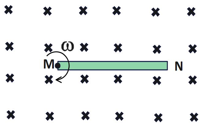
2.A metallic rod MN of length ℓ is rotated with angular velocity \omega about an axis passing through one of its end and perpendicular to the plane of the paper, in uniform magnetic field \overrightarrow B as shown in figure. Derive an expression for the induced emf (motional e.m.f.) developed between the end points M and N.

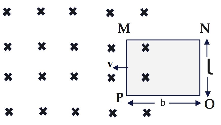
3. The figure shows a rectangular conducting frame MNOP of resistance R placed partly in a perpendicular magnetic field \overrightarrow B and moved with velocity \overrightarrow v as shown in the figure. 

Important Physics derivations for Board Examinations

Obtain the expressions for the

(a) induced current in the loop

(b) force acting on the arm ‘ON’ and its direction, and

(c) power required to move the frame to get a steady emf induced between the arms MN and PO.

4.Two concentic circular coils X and Y of radii r_1 and r_2 (r_1>>r_2) having N_1 and N_2 turns respectively are placed coaxially with centres coinciding. Obtain an expression for
(i) the mutual inductance for the arrangement, and
(ii) the magnetic flux linked with coil Y when current I flows through coil X.

5.Obtain the expression for the mutual inductance of two long co-axial solenoids S_1 and S_2 wound one over the other , each of length L and radii r_1 and r_2 and n_1 and n_2 number of turns per unit length , when a current I is set up in the outer solenoid S_2

6. Define self-inductance of a coil. Derive the expression for magnetic energy stored in an inductor L connected across a source of emf to build up a current I through it.

7.Define self-inductance of a coil. Derive the expression for self-inductance of a solenoid of length L and  and r, having N turns. 

8. A rectangular coil of area A, having number of turns N is rotated at ‘f ‘ revolutions per second in a uniform magnetic field B, the field being perpendicular to the coil. Prove that the maximum emf induced in the coil is 2\pi fBAN

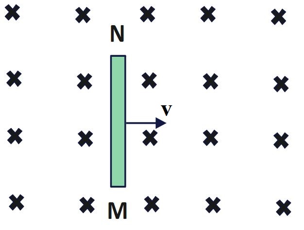
9.A metallic rod MN of length ℓ moves with linear velocity \overrightarrow v , perpendicular to uniform magnetic field \overrightarrow B as shown in figure. Derive an expression for the induced emf (motional e.m.f.) developed between the end points M and N.
Important Physics derivations for Board Examinations

Important Physics derivations for Board Examinations

Chapter 5 – Magnetism and Magnetic Materials

1.Derive relationship (\mu_{r\;}=\;1+\;\chi_m) between magnetic susceptibility \chi_m and relative permeability \mu_r.

2. Show that a current carrying solenoid is as equivalent to a tiny bar magnet.

Important Physics derivations for Board Examinations

Chapter 4 – Moving Charges and Magnetism

1. Using Biot-Savarat law, derive an expression for the magnitude of the magnetic field at a distance radius ‘r’ from a finite straight wire carrying current ‘I’. Also, deduce the magnetic field due infinitely long straight wire. 

2.(i) State Biot – Savart law in vector form expressing the magnetic field\overrightarrow B due to an element \overrightarrow {dl} carrying current I at a distance \overrightarrow r from the element.

(ii) Derive an expression for the magnitude of the magnetic field at the centre of a circular loop of radius r carrying a steady current I. Draw the field lines due to the current loop.

3. Use Biot-Savart law to derive the expression for magnetic field B at a point P on the axis (distance x from centre) of a circular coil of radius ‘r’ carrying current ‘I’ and hence find the magnetic field at the centre ‘O’ of the circular coil carrying current.

4. Using Ampere’s circuital law, obtain an expression for the magnetic field due a infinitely long straight wire carrying current ‘I’.

5.Using Ampere’s circuital law, obtain an expression for the magnetic field along the axis of a current carrying solenoid of length l and having N number of turns.

6.Derive the expression for force per unit length between two long straight parallel current carrying conductors. Hence define one ampere.

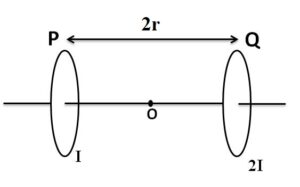
7.Two identical circular loops, P and Q, each of radius r and carrying current I and 2I respectively are lying in parallel planes such that they have a common axis. The direction of current in both the loops is clockwise as seen from O which is equidistant from both the loops. Obtain the expression for the magnitude of the net magnetic field at point O.

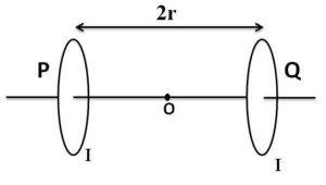
8.Two identical circular loops, P and Q, each of radius r and carrying equal currents are kept in the parallel planes having a common axis passing through O. The direction of current in P is clockwise and in Q is anti-clockwise as seen from O which is equidistant from the loops P and Q. Obtain the expression for the magnitude of the net magnetic field at O.

9. A rectangular coil PQRS of sides ‘l’ and ‘b’ carrying a current I is subjected to a uniform magnetic field \overrightarrow B  acting perpendicular to its plane. Obtain the expression for the torque acting on it.

10.Deduce the expression for the magnetic dipole moment of an electron orbiting around the central nucleus.

11.Describe the working principle of a moving coil galvanometer. Why is it necessary to use
(i) a radial magnetic field and
(ii) a cylindrical soft iron core in a galvanometer? Write the expression for current sensitivity of the galvanometer.
Can a galvanometer as such be used for measuring the current?

12.(a) Discuss the conversion of galvanometer  to  ammeter which can measure current ranging from 0 to I. Deduce the expression for ammeter current I if galvanometer can allow maximum current  I_g to pass through itself.

(b) Explain, giving reasons, the basic difference in converting a galvanometer into
(i) a voltmeter and
(ii) an ammeter.

13.(a) Discuss the conversion of galvanometer  to  voltmeter which can measure voltage ranging from 0 to V. Deduce the expression for  potential difference V that it can measure  if galvanometer can allow maximum current  I_g to pass through itself.

(b) Explain, giving reasons, the basic difference in converting a galvanometer into
(i) a voltmeter and
(ii) an ammeter.

14.(a) Use Biot-Savart law to derive the expression for the magnetic field due to a circular coil of radius R having N turns at a point on the axis at a distance ‘x’ from its centre. Draw the magnetic field lines due to this coil.
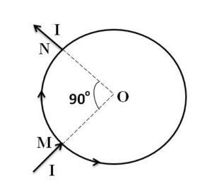
(b) A current ‘I’ enters a uniform circular loop of radius ‘R’ at point M and flows out at N as shown in the figure.

Obtain the net magnetic field at the centre of the loop.

Important Physics derivations for Board Examinations

Chapter 3 – Current Electricity

1.Derive an expression for drift velocity of free electrons in a conductor in terms of relaxation time.

2.Explain the term ‘drift velocity’ of electrons in a conductor. Hence obtain the expression for the current through a conductor in terms of ‘drift velocity’

3.Derive an expression for the resistivity of a good conductor, in terms of the relaxation time of electrons.

4.(i) Define the term drift velocity.
(ii) On the basis of electron drift, derive an expression for resistivity of a conductor in terms of number density of free electrons and relaxation time. On what factors does resistivity of a conductor depend? 
             (OR)
Derive an expression for the resistivity \rho=\frac m{ne^2\tau} a good conductor, in terms of the relaxation time of electrons.

5.Use Kirchhoff’s rules to derive conditions for the balanced Wheatstone bridge.

6.Using the concept of drift velocity of charge carriers in a conductor, deduce the relationship between current density and resistivity/conductivity of the conductor. 

7.Derive an expression for the current density of a conductor in terms of the drift speed of electrons. 

8.A number of identical cells n, each of emf e, internal resistance r connected in series are charged by a d.c. source of emf elr using a resistor R.
(i) Draw the circuit arrangement.
(ii) Deduce the expressions for
(a) the charging current and (b) the potential difference across the combination of the cells.

9.Find the relation between drift velocity and relaxation time of charge carriers in a conductor. A conductor of length L is connected to a d,c. source of emf ‘E’. If the length of the conductor is tripled by stretching it, keeping ‘E’ constant, explain how its drift velocity would be affected.

Important Physics derivations for Board Examinations

Chapter 2 – Electrostatic Potential and Capacitance

1.Derive an expression for capacitance of isolated spherical conductor.

2. Derive the expression for the capacitance of a parallel plate capacitor having plate area A and plate separation d.

3.Derive an expression for capacitance of parallel plate capacitor completely filled with dielectric of dielectric constant K.

4.Derive an expression for capacitance of parallel plate capacitor partially filled with dielectric of width t (t < d).

5.Explain using suitable diagrams, the difference in the behavior of a (a) conductor and (b) Dielectric in the presence of external electric field. Define the polarization of dielectric and write its relation with susceptibility. Also derive relationship between susceptibility and dielectric constant.

6. Derive an expression for potential at any point P on axial line of dipole of length ‘2a’ at a distance ‘r’ from the center of dipole. Also deduce the potential for short dipole. 

7. Derive an relationship between electric field and potential gradient, E = – dV/dr

8.Show that the potential at any point on equatorial line of a dipole at a distance ‘r’ from the center of dipole is zero. 

Important Physics derivations for Board Examinations

Chapter 1 – Electric Charges and Fields

1.Derive an expression for electric field intensity at any point P on axial line of dipole of length ‘2a’ at a distance ‘r’ from the center of dipole. Also deduce the electric field intensity for short dipole. 

2.Derive an expression for electric field intensity at any point P on equatorial line of dipole of length ‘2a’ at a distance ‘r’ from the center of dipole. Also deduce the electric field intensity for short dipole. 

3.Derive an expression for electric field intensity due to short dipole at any general point at a distance ‘r’ from the dipole of dipole moment \overrightarrow p .

4. Derive an expression for torque acting on electric dipole  placed in uniform electric field \overrightarrow E . Also , explain the stable and unstable equilibrium of dipole position on the basis of torque experienced by it. 

5.Derive an expression for electrostatic potential energy of  electric dipole  placed in uniform electric field \overrightarrow E . Also , explain the stable and unstable equilibrium of dipole position on the basis of P.E. of dipole.

6. Using Gauss’ Law , derive an expression for electric field intensity due to uniformly charged infinitely long straight wire having linear charge density ‘\lambda‘ at a distance r from it.

7.Using Gauss’ Law , derive an expression for electric field intensity due to uniformly charged infinite thin sheet having surface charge density ‘\rho

8.Derive an expression for the electric field due to a uniformly charged thin spherical shell (i) outside the shell and (ii) inside the shell using Gauss’s law. Also draw required graph showing variation of electric field with distance from the center of spherical shell.

Now, we have gone through frequently asked "Important Physics derivations" in CBSE Board Examinations. Click here to know more essential topics related to Electromagnetism.

Kinematics: Understanding Uniform Motion

Kinematics: Understanding Uniform Motion

Kinematics: Understanding Uniform Motion

What is Kinematics 

Kinematics is the branch of physics that deals with the motion of objects without considering the causes of motion. Among the various types of motion, uniform motion is a fundamental concept that provides a foundation for understanding more complex movements. In this article, we will delve into the intricacies of uniform motion, explore its characteristics, and see its applications in our daily lives.

What is Uniform Motion?

Uniform motion refers to the movement of an object at a constant speed in a straight line along specific fixed direction. In other words, the object covers equal distances in equal intervals of time, regardless of how small these intervals might be. This type of motion is characterized by:

  • Constant Velocity: The speed/magnitude of velocity and direction of the object’s motion remain unchanged.
  • Zero Acceleration: Since the velocity is constant, there is no change in speed or direction, resulting in zero acceleration.

As , \overrightarrow{v\;}\;=\;constan t\;

Therefore, \overrightarrow{a\;}=\;\frac{d\overrightarrow v}{dt}=\;0

Mathematical Representation

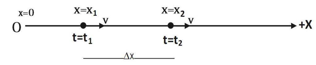
Consider an object is moving along +X axis with uniform velocity ‘v’ as shown in diagram. Assume that object is at position x=x_1 at time t=t_1 and reaches at position x=x_2 at time t=t_2

Kinematics: Understanding Uniform Motion

We know that velocity of object is defined as rate change of position of object w.r.t. time. Mathematically,

v=\frac{dx}{dt}\;

\Rightarrow dx\;=\;v\;dt\;

\int_{x_1}^{x_2}dx\;=\;\int_{t_1}^{t_2}v\;dt\;

\int_{x_1}^{x_2}dx\;=\;v\int_{t_1}^{t_2}\;dt\; (v= constant/uniform)

\left|x\right|_{x_1}^{x_2}=\;v\;\left|\;t\;\right|_{t_1}^{t_2}

x_2\;-x_1\;=\;v\;(t_2-t_1)

\Delta x\;=v\;\Delta t

v=\frac{\Delta x}{\Delta t}

Hence,\;v=\frac{dx}{dt}=\frac{\Delta x}{\Delta t}=constant

Clearly, uniform motion reflects that the object covers equal distances in equal intervals of time, regardless of how small these intervals might be.

When object/particle starts motion from origin (x=0)

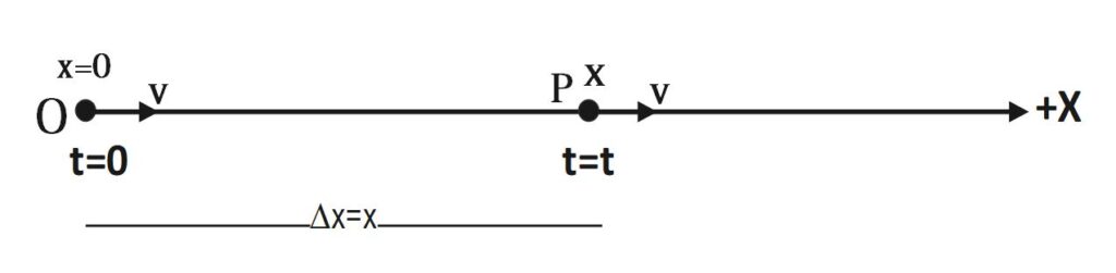
When particle starts motion from origin then initial displacement of particle is zero i.e. at t= 0 , x=0 . And it moves with constant velocity v, finally reaches at P in time t. Thus, at time t = t , x = x as shown in following diagram .

We know that for uniform motion, 

\Delta x\;=v\;\Delta t

x-0= v(t-0)

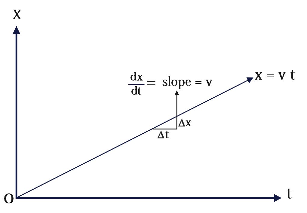
x = v t

Kinematics: Understanding Uniform Motion

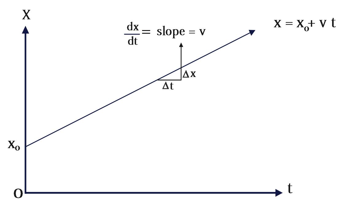
Position-Time (x-t) graph of uniform motion starting from origin

Kinematics: Understanding Uniform Motion

When object/particle starts motion with some initial displacement

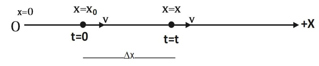
When particle does not starts motion from origin but from x= x_o then initial displacement of particle is non-zero i.e. at t=0 , x= x_o  .  With constant velocity v, it finally reaches at position x in time t as shown in following diagram . Thus, at time t = t , x = x 

We know that for uniform motion, 

\Delta x\;=v\;\Delta t

x-x_o= v(t-0)

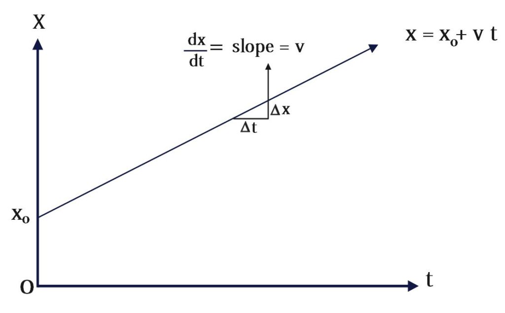
x = x_o+ v t

Kinematics: Understanding Uniform Motion

Position-Time(x-t) graph of uniform motion of particle with non-zero initial displacement

Kinematics: Understanding Uniform Motion

Graphical Representation

Position-Time Graph

In a distance-time graph for uniform motion, the distance (y-axis) plotted against time (x-axis) yields a straight line with a constant slope. The slope of this line equals the velocity of the object.

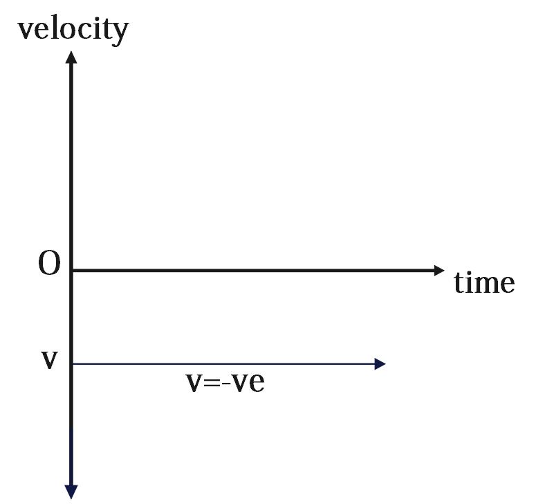
Velocity-Time Graph

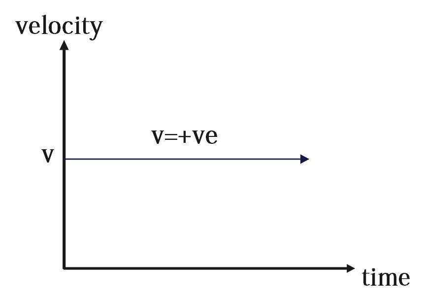
In a velocity-time graph for uniform motion, the velocity (y-axis) plotted against time (x-axis) is a straight horizontal line. This horizontal line indicates that the velocity remains constant over time.

Kinematics: Understanding Uniform Motion

Uniform Motion vs. Non-Uniform Motion

Understanding the difference between uniform and non-uniform motion is crucial. While uniform motion features a constant velocity, non-uniform motion involves a change in speed or direction, indicating acceleration. Real-world motions are often non-uniform due to varying forces acting on objects, but uniform motion serves as an idealized model to simplify analysis.

Conclusion

Uniform motion, with its simplicity and predictability, is a cornerstone concept in kinematics. It lays the groundwork for more complex analyses of motion in physics and engineering. By grasping the fundamentals of uniform motion, one can better understand the intricate dynamics of moving objects, both in theoretical contexts and real-world applications. Whether it’s a car cruising on a highway or the precise movement of a spacecraft, uniform motion continues to be a vital principle in the study of mechanics.

Force between the plates of charged capacitor

Force between the plates of capacitor

Force between the plates of capacitor

Introduction

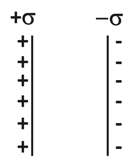
Capacitors are fundamental components in electronics, used to store electrical energy. When a voltage is applied across the plates, an electric field develops, causing a charge to accumulate on the plates. The capacitor stores energy in the electric field created between the plates.

Among various types of capacitors, the parallel plate capacitor is one of the simplest and most widely studied. Understanding the force between the plates of a charged parallel plate capacitor not only deepens our comprehension of electrostatic principles but also has practical applications in various technologies.

Derivation of Force between the Plates of Capacitor

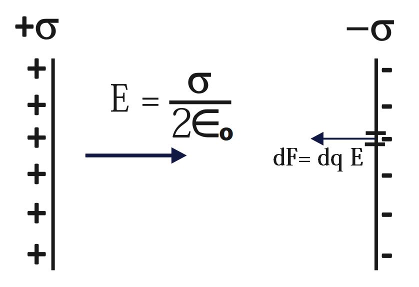
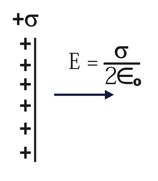
To derive the force between the plates, let us consider the small element of charge dq on second plate. Thus, calculate the force of attraction due to the electric field (of first plate) on small element of charge on second plate (-vely charged). 

We already know that,
E=\;\frac\sigma{2\in_o} 
Force between the plates of capacitor
Force due to uniform electric field E on small element dq
dF\;=\;dq\;E  
Integrating both sides
\int dF\;=\;\int dq\;E  
F\;=\;E\;\int dq\; (As, E = constant)
F\;=\;E\;q
F\;=\;\left(\frac\sigma{2\in_o}\right)\;q
F\;=\;\left(\frac q{2A\in_o}\right)\;q
F\;=\frac{q^2}{2A\in_o}
Hence, we have obtained that the formula of force between the plates of capacitor
F\;=\frac{q^2}{2A\in_o}

Practical Implications

Understanding of the force between the plates of a capacitor is crucial for several reasons:

  1. Mechanical Stability: In high-voltage applications, the force can be significant, potentially leading to mechanical deformation or even damage if the capacitor is not designed to handle such forces.

  2. Design Considerations: Engineers need to consider this force when designing capacitors to ensure they remain stable and functional under varying electrical conditions.

  3. Microelectromechanical Systems (MEMS): In MEMS devices, capacitors can be used as actuators where the force between plates is used to move microstructures.

Transient Current : Charging of Capacitor

Transient Current: Charging of Capacitor with DC source

Charging of Capacitor with DC source - IIT Advanced Topic

Transient Current :

Transient current is a temporary current that flows for a short, finite duration, starting from zero to a maximum value or from a maximum value to zero, in response to a sudden change in the circuit conditions, such as when a switch is turned on or off.

Charging of Capacitor : Introduction

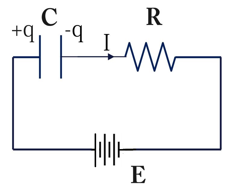
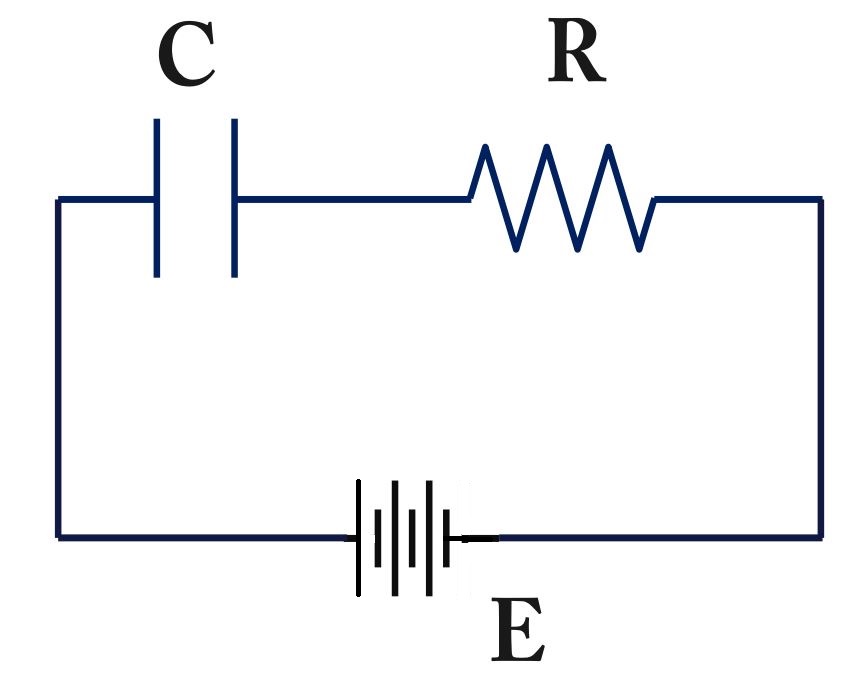
Capacitor with DC source is practically CR circuit. In the capacitor charging there are three stages:

  1. Initial Condition:

    • When an uncharged capacitor is connected to a voltage source through a resistor, the transient current initially flows from zero to a maximum value.
  2. Exponential Decay:

    • The current then decreases exponentially over time as the capacitor charges, described by the equation:
      I(t)\;=\;I_o\;e^{-\frac t{CR}}
      where E is the applied voltage, is the resistance, is the capacitance, and 𝑡 is the time elapsed.
  3. Steady State:

    • Once the capacitor is fully charged, the current drops to zero, indicating the end of the transient period. 
      I\;=\;\frac{dq_0}{dt}=\;o\;
Initial Condition
Transient Current: Charging of Capacitor with DC source
When switch is just closed, time, t=0 and capicitor is uncharged . So, Charge q=0
Also, intially the current will be maximum.
hence, I_o=\;\frac ER
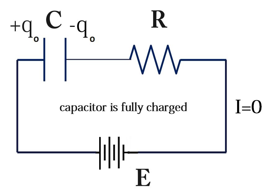
Steady State
Transient Current: Charging of Capacitor with DC source
Capacitor continues getting charged until it is fully charged . This is called steady state.

As, we know that 

I\;=\;\frac{dq_0}{dt}=\;o\; 

where q_o is maximum charge

Therefore, according to Kirchhoff’s loop rule

E\;-\;\frac{q_o}C-(0)\;R=\;0


E\;-\;\frac{q_o}C=\;0


E\;=\;\frac{q_o}C


q_o\;=\;EC…….(1)


Assume that capacitor is charged up to charge q at any time t.
Therefore, time = t and charge = q
According to Kirchhoff's loop rule,
E-\;\frac qC-IR\;=\;0
EC-q-ICR\;=\;0
EC-q-\frac{dq}{dt}\;(CR)\;=\;0
q_o-q-\frac{dq}{dt}\;(CR)\;=\;0 [from(1)]
\frac{q_0-q}{CR}-\;\frac{dq}{dt}=0
\frac{q_0-q}{CR}=\;\frac{dq}{dt}
\frac1{CR}\;dt\;=\;\frac{dq}{q_o-q}\;
Integrating both sides
\int_0^t\frac1{CR}\;dt\;=\;\int_0^q\frac{dq}{q_o-q}\;
\frac1{CR}\int_0^t\;dt\;=\;\int_0^q\frac{dq}{q_o-q}\;
\frac1{CR}\;\left|t\right|_0^t\;\;=\;\;\left|\frac{\log_e\left(q_o-q\right)}{-1}\right|_0^q
\frac1{CR}(t-0)\;\;=\;\;-\;\lbrack\log_e\left(q_o-q\right)-\;\log_e\left(q_o-0\right)\rbrack
-\frac t{CR}\;=\;\;\;\log_e\left(\frac{q_o-q}{q_o}\right)
e^{-\frac t{CR}\;}\;=\;\frac{q_o-q}{q_o}
q_o\;e^{-\frac t{CR}\;}\;=\;q_o-q
\;q=q_o-\;q_o\;e^{-\frac t{CR}\;}\;
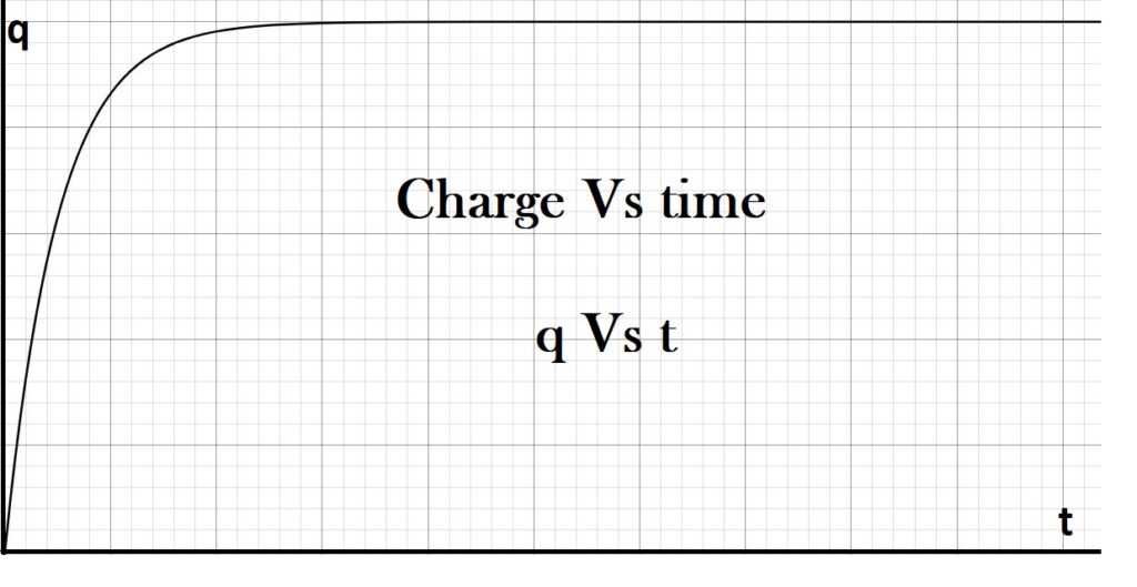
\;q=q_o(1-\;\;e^{-\frac t{CR}\;}\;)
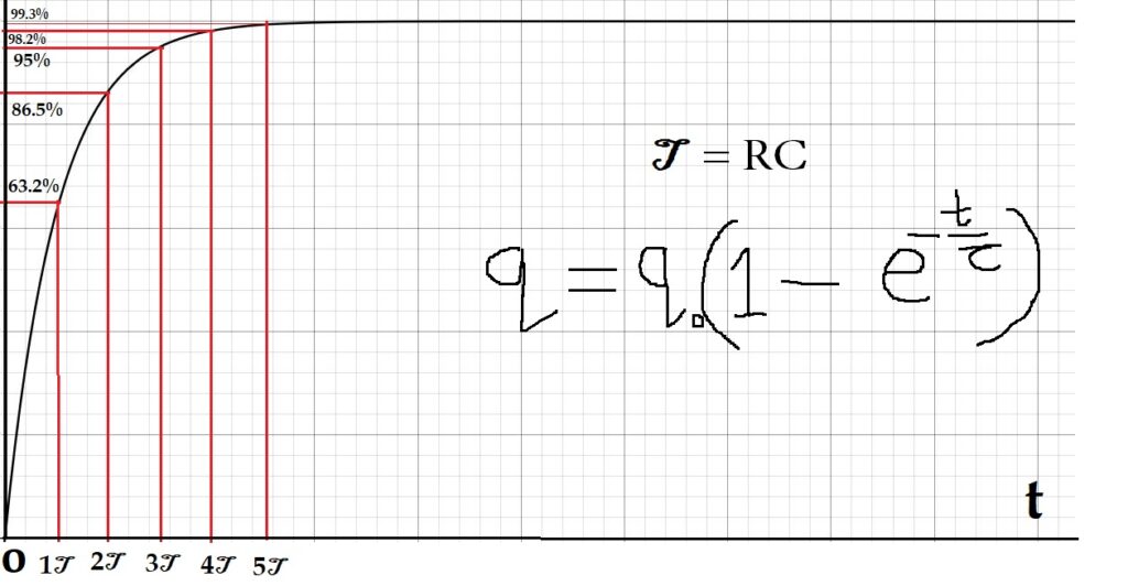
q=\;q_o\;(1-e^{-\frac t\tau})
\tau = CR is called Time Constant

When time t=\;1\;\tau

So, q=\;q_o(1-\;e^{-1})\;=\;0.632\;q_o

Capacitor gets charged by 63.2% in first time constant

When time t=\;2\;\tau

So, q=\;q_o(1-\;e^{-2})\;=\;0.865\;q_o

Capacitor gets charged by 86.5% in two time constants

When time t=\;3\;\tau

So, q=\;q_o(1-\;e^{-3})\;=\;0.950\;q_o

Capacitor gets charged by 95% in three time constants

When time t=\;4\;\tau

So, q=\;q_o(1-\;e^{-4})\;=\;0.982\;q_o

Capacitor gets charged by 98.2% in four time constants

When time t=\;5\;\tau

So, q=\;q_o(1-\;e^{-5})\;=\;0.993\;q_o

Capacitor gets charged by 99.3% in five time constants

When steady state is attained, capacitor is fully charged

t\;\rightarrow\infty

q=\;q_o(1-\;e^{-\infty})\;

q=\;q_o(1-\;0)=\;q_o

So, q=\;q_o

\;q=q_o(1-\;\;e^{-\frac t{CR}\;}\;)
taking derivative both sides w.r.t. t
\frac{dq}{dt}=q_o\;\frac d{dt}(1-\;e^{-\frac t{CR}})
\frac{dq}{dt}=q_o\;\lbrack\;0-\;e^{-\frac t{CR}}\;\times\;(-\frac1{CR}\;)\;\rbrack
\frac{dq}{dt}=\;\frac{q_o}{RC}\;\;e^{-\frac t{CR}}\;
\frac{dq}{dt}=\;\frac{EC}{RC}\;\times\;e^{-\frac t{CR}}\;
\frac{dq}{dt}=\;\;\frac ER\;\times\;e^{-\frac t{CR}}\;
I=\;\;I_o\;\times\;e^{-\frac t{CR}}\; [ From (1) ]
I=\;\;I_o\;\;e^{-\frac t{CR}}\;

Exponential Growth of Charge : Charging of Capacitor

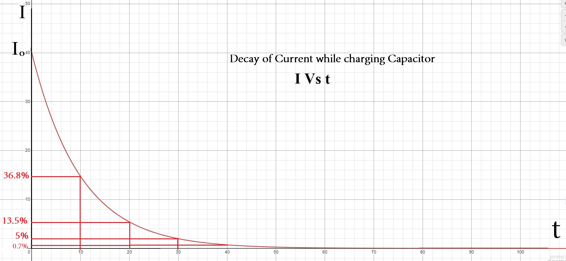
Exponential Decay of Current : Charging of Capacitor

I=\;\;I_o\;\;e^{-\frac t{CR}}\;

I=\;I_o\;e^{-\frac t\tau}

I=\;I_o\;e^{-\frac t\tau}

When time t=\;1\;\tau

I=\;\;I_o\;e^{-1}\;

I=\;0.368\;I_o\;

So, current reduces by 62.8% of maximum current in 1 time constant

When time t=\;2\;\tau

I=\;\;I_o\;e^{-2}\;

I=\;0.135\;I_o\;

So, current reduces by 86.5% of maximum current in 2 time constants

When time t=\;3\;\tau

I=\;\;I_o\;e^{-3}\;

I=\;0.05\;I_o\;

So, current reduces by 95% of maximum current in 3 time constants

When time t=\;4\;\tau

I=\;\;I_o\;e^{-4}\;

I=\;0.018\;I_o\;

So, current reduces by 98.2% of maximum current in 3 time constants

When time t=\;5\;\tau

I=\;\;I_o\;e^{-5}\;

I=\;0.07\;I_o\;

So, current reduces by 99.3% of maximum current in 3 time constants

When steady state is achieved , then current reduces to zero

t\;\rightarrow\infty

I=\;\;I_o\;e^{-\infty}\; =0

Charging of Capacitor : An Overview

Initially, when switched is just on ,  capacitor is is uncharged and it offers zero resistance to DC source and current is maximum(largest possible). Thus, we can calculate the value of maximum current by formula,  I_o=\;\frac ER 

Finally, steady state is attained after some time (theoretically , when  t\;\rightarrow\infty ) and capacitor gets fully charged. Now, capacitor starts blocking DC (direct current) and it reduces to zero i.e. I = 0

Consequently, maximum charge is q_o\;=\;EC

During charging of capacitor , current falls from I_o to 0 . This is known as decay of current. It is found that the decay of current is exponential decay as according to formula  I=\;\;I_o\;\;e^{-\frac t{CR}}\;      

Numerical based on Charging of Capacitor

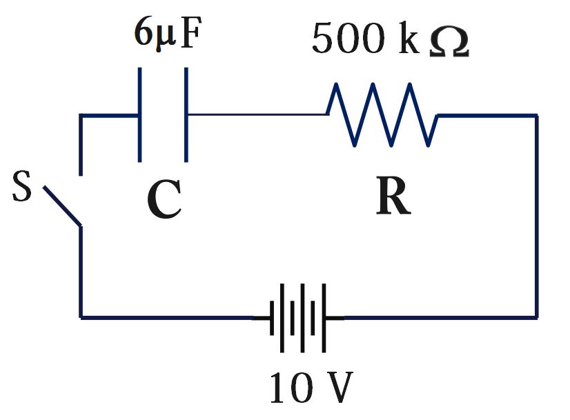
Ex. An uncharged capacitor and a resistor are connected in series, as shown in the figure below. The emf of the battery is ε = 10 V, C = 6 μF, and R = 500 kΩ.

After the switch is closed, find

(a) The time constant of the RC circuit.

(b) The maximum charge on the capacitor.

(c) The charge on the capacitor 6 s after the switch is closed.

(d) The charge on the capacitor 8.1 s after the switch is closed.

Solution:

(a) Time Constant, \tau = CR
\tau\;\;=\;6\mu\;\times\;500\;k=\;6\;\times10^{-6}\;\times\;500\;\times10^3
\tau\;\;=\ 3 s
(b) The maximum charge on the capacitor
Charge wll be maximum when steady state is achieved and capacitor gets fully charged, q_o=\;C\;E
q_o=\;6\times10^{-6}\times10\;=\;60\;\mu C
q_o =\;60\;\mu C
(c) The charge on the capacitor 6 s after the switch is closed.
Charge on capacitor at any instant t, q=\;q_o\;(1-e^{-\frac t\tau})
q(t)=\;q_o\;(1-e^{-\frac t\tau})
q(6)=\;q_o\;(1-e^{-\frac 63})
q(6)=\;60\;(1-e^{-2})
q(6)=\;60\;(1-0.135)
q(6)=\;60\;(0.865)
q(6)\;=\;51.9\;\mu C\;\approx\;52\;\mu C\;
q(6)\;=\;52\;\mu C\;
(d) The charge on the capacitor 8.1 s after the switch is closed.
Charge on capacitor at any instant t, q=\;q_o\;(1-e^{-\frac t\tau})
q(t)=\;q_o\;(1-e^{-\frac t\tau})
q(8.1)=\;q_o\;(1-e^{-\frac {8.1}3})
q(8.1)=\;60\;(1-e^{-2.7})
q(8.1)=\;60\;(1-0.067)
q(8.1)=\;60\;(0.933)
q(8.1)\;=\;55.98\;\mu C\;\approx\;56\;\mu C\;
q(8.1)\;=\;56\;\mu C\;

Electrostatics-10 Important basic MCQs (Quiz) Part 3

Electrostatics-10 Important basic MCQs (Quiz) Part 3

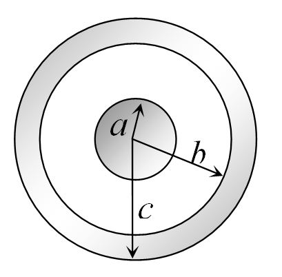
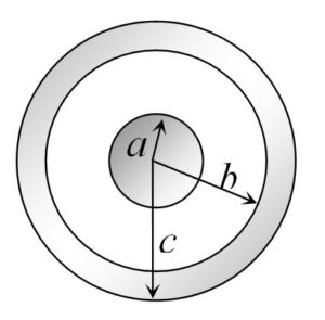
1. A solid conducting sphere of radius a has a net positive charge 2Q. A conducting spherical shell of inner radius and outer radius c is concentric with the solid sphere and has a net charge – Q. The surface charge density on the inner and outer surfaces of the spherical shell will be 

Electrostatics-10 Important basic MCQs (Quiz) Part 3

(A) -\frac{2Q}{4\mathrm{πb}^2},\;\frac Q{4\mathrm\pi\;\mathrm c^2}

(B) -\frac{Q}{4\mathrm{πb}^2},\;\frac Q{4\mathrm\pi\;\mathrm c^2}

 (C) 0, \frac Q{4\mathrm\pi\;\mathrm c^2}

(D) None of the above

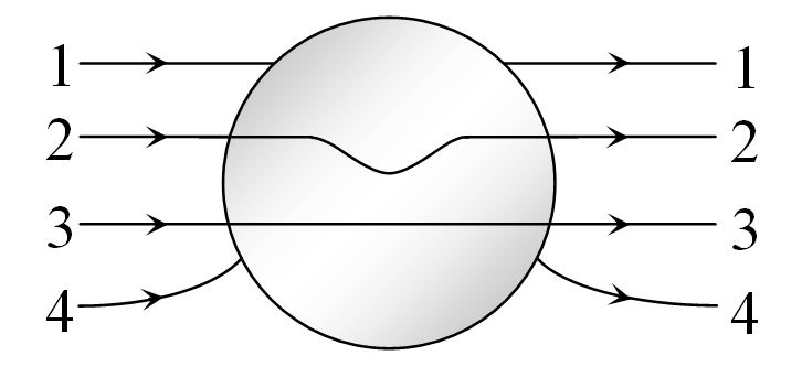
2. A metallic solid sphere is placed in a uniform electric field. The lines of force follow the path(s) shown in figure as:

Electrostatics-10 Important basic MCQs (Quiz) Part 3

(A)   1   

(B)  2

 (C) 3                              

(D) 4

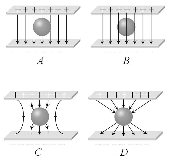
3.An uncharged sphere of metal is placed in between two charged plates as shown. The lines of force look like

Electrostatics-10 Important basic MCQs (Quiz) Part 3

(A) A                     

(B) B

(C) C                      

(D) D

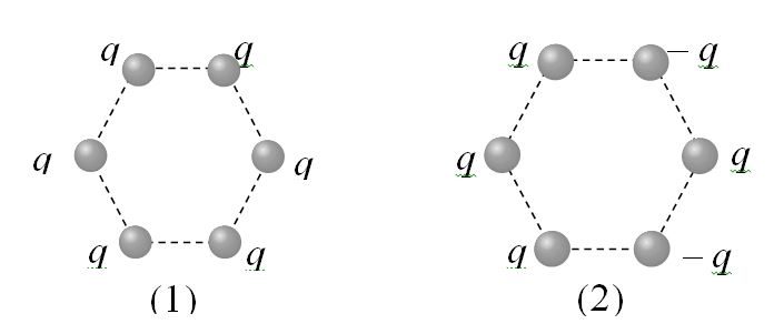
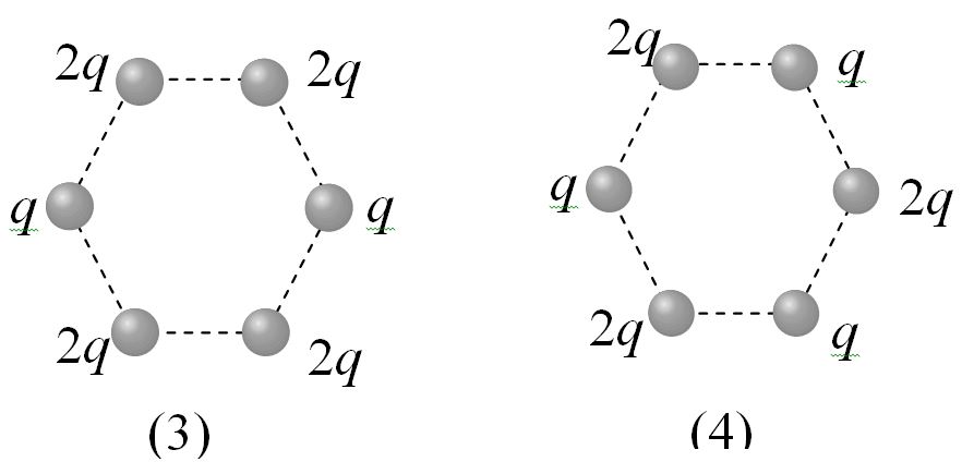
4.Figures below show regular hexagons, with charges at the vertices. In which of the following cases the electric field at the centre is not zero

(A) 1                                       

(B) 2

(C) 3                             

(D) 4

5. Two point charges +8q and -2q  are located at x=0  and  x=L respectively.  The location of a point on the x-axis at which the net electric field due to these two point charges is zero is

(A) 8 L                           

(B) 4 L

(C) 2 L                           

(D) \frac L4


6. At a certain distance from a point charge the electric field is 500 V/m and the potential is 3000V/m . What is this distance

(A)  6m                         

(B) 12m

(C) 36m                       

 (D) 144m

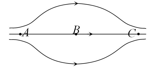
7. The figure shows some of the electric field lines corresponding to an electric field. The figure suggests

(A)E_A>\;E_B>\;E_C                

(B) E_A=\;E_B=\;E_C 

(C) E_A=\;E_C>\;E_B                

(D) E_A=\;E_C<\;E_B   

8. Point charges +4q, -q and +4q are kept on the axis at points x=0, x=a and  x=2a respectively, then

(A) Only  ‘-q’ is in stable equilibrium

(B) None of the charges are in equilibrium

(C) All the charges are in unstable equilibrium

(D) All the charges are in stable equilibrium

9. Two point charges of 20\;\mu C\; and 80\;\mu C\;  are   10 cm  apart. Where will the electric field strength be zero on the line joining the charges from 20\;\mu C\; charge

(A) 0.1 m                         

(B)0.033 m 

(C) 0.33 m                

(D) 0.04 m

10. What is the magnitude of a point charge which produces an electric field of 2 N/coulomb at a distance of 60 cm 

(A) 8\;\times\;10^{-11}\;C

(B) 2\;\times\;10^{-12}\;C

(C) 3\;\times\;10^{-11}\;C

(D) 6\;\times\;10^{-10}\;C


Electrostatics-10 Important basic MCQs (Quiz) Part 1

Electrostatics-10 Important basic MCQs (Quiz) Part 2

Electrostatics-10 Important basic MCQs (Quiz) Part 2

Electrostatics-10 Important basic MCQs (Quiz) Part 2

Electrostatics-10 Important basic MCQs (Quiz) Part 2

1.ABC is a right angled triangle in which AB= 3 cm  and BC = 4cm  . And \angle ABC\;=\frac{\mathrm\pi}2 . The three charges +15, +12    and  -20 e.s.u. are placed respectively on  A, B  and C . The force acting on B is 

(A) 125 dyne

(B) 35 dynes

 (C) 25 dynes

(D) Zero

2.Electric charges of 1\mu C, -1\mu C and 2\mu C  are placed in air at the corners A, B and C respectively of an equilateral triangle ABC having length of each side 10 cm. The resultant force on the charge at C is

(A) 0.9 N                       

(B) 1.8 N

(C) 2.7 N                       

(D) 3.6 N

3. Two charges placed in air repel each other by a force of 10^{-4} N . When oil is introduced between the charges, the force becomes 2.5\;\times\;10^{-5}\;N.The dielectric constant of oil is

(A) 2.5                         

B) 0.25

(C) 2.0                           

(D) 4.0

4. Two spherical conductors B and C having equal radii and carrying equal charges in them repel each other with a force F when kept apart at some distance. A third spherical conductor having same radius as that of B but uncharged is brought in contact with B, then brought in contact with C and finally removed away from both. The new force of repulsion between B and C is

 (A) F/4                         

(B) 3F/4

(C) F/8                

(D) 3F/8

5. The charges on two sphere are +7µC and –5µC They experience a force F. If each of them is given and additional charge of – 2µC, the new force of attraction will be

 (A) F                             

(B) F / 2

(C)  \frac F{\sqrt3}                 

(D) 2F

6. Electric lines of force about negative point charge are

(A) Circular, anticlockwise  

(B) Circular, clockwise

(C) Radial, inward

(D) Radial, outward

7. A charge q is placed at the centre of the line joining two equal charges  Q. The system of the three charges will be equilibrium, if  is equal to

(A) -\frac Q2                          

(B)-\frac Q4    

(C) +\frac Q4                             

(D) +\frac Q2    

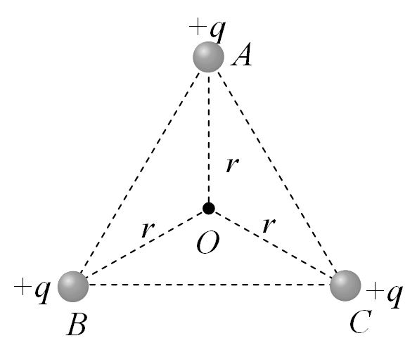
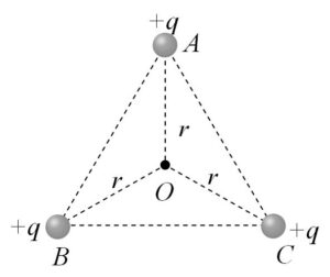
8. ABC is an equilateral triangle. Charges +q are placed at each corner. The electric intensity at O will be

Electrostatics-10 Important basic MCQs (Quiz) Part 2

 (A)\frac1{4\mathrm\pi\;\in_{\mathrm o}}\frac q{r^2}

(B)\frac1{4\mathrm\pi\;\in_{\mathrm o}}\frac{3q}{r^2}

(C) Zero

(D)\frac1{4\mathrm\pi\;\in_{\mathrm o}}\frac qr

9. The electric field inside a spherical shell of uniform surface charge density is

(A) Zero

(B) Constant, less than zero

(C) Directly proportional to the distance from the centre

 (D) None of the above

10.When a body is earth connected, electrons from the earth flow into the body. This means the body is…..

 (A) Unchanged

(B) Charged positively

(C) Charged negatively  

(D) An insulator

Electrostatics-10 Important basic MCQs (Quiz) Part 1

Electrostatics-10 Important basic MCQs (Quiz) Part 1

Electrostatics-10 Important basic MCQs (Quiz) Part 1

1.An isolated solid metallic sphere is given charge +Q.  The charge will be distributed on the sphere       

 (A) Uniformly but only on surface

(B) Only on surface but non-uniformly

(C) Uniformly inside the volume

(D) Non-uniformly inside the volume

2. Four charges are arranged at the corners of a square ABCD, as shown in the adjoining figure. The force on the charge kept at the centre O is

Electrostatics-10 Important basic MCQs (Quiz) Part 1

(A) Zero

(B) Along the diagonal AC

(C) Along the diagonal BD

(D) Perpendicular to side AB

3.The ratio of the forces between two small spheres with constant charge in (a) air  (b) in a medium of dielectric constant K is
(A) 1 : K                        

(B) K : 1

(C) 1: K^2  

(D) K^2 : 1     

4. Three charges 4q , Q and q  are in a straight line in the position of 0, l/2,  and l respectively.   The resultant force on q will be zero, if  Q=

(A) – q                           

(B) – 2q

(C) -\frac q2 

(D)  4q

5.Two charges each of 1 coulomb are at a distance 1 km apart, the force between them is  

(A)     9\;\times\;10^3\;Newton\;         

(B) 9\;\times\;10^{-3}\;Newton\;  

(C) 1.1\;\times\;10^{-4}\;Newton\;

(D) 10^4\;Newton\;  

6. There are two metallic spheres of same radii but one is solid and the other is hollow, then

 (A) Solid sphere can be given more charge

 (B) Hollow sphere can be given more charge

(C) They can be charged equally (maximum)

(D) None of the above

7. Three equal charges are placed on the three corners of a square. If the force between q_1 and q_2 is F_{12}  and that between q_1  and q_3 is F_{13} , the ratio of magnitudes \frac{F_{12}}{F_{13}} is 

(A) \frac12                     

(B) 2 

(C)  \frac1{\sqrt2}\;

(D) \sqrt{2\;} 

8. Two small spheres each having the charge Q are suspended by insulating threads of length  from a hook. This arrangement is taken in space where there is no gravitational effect, then the angle between the two suspensions and the tension in each will be

(A) 180^o,\;\frac1{4\mathrm\pi\;\in_{\mathrm o}}\frac{Q^2}{{(2L)}^2}   

(B)   90^o,\;\frac1{4\mathrm\pi\;\in_{\mathrm o}}\frac{Q^2}{{L}^2}

(C)    180^o,\;\frac1{4\mathrm\pi\;\in_{\mathrm o}}\frac{Q^2}{2 L^2}           

(D)    180^o,\;\frac1{4\mathrm\pi\;\in_{\mathrm o}}\frac{Q^2}{  L^2}           

9. A soap bubble is given a negative charge, then its radius

(A) Decreases

(B) Increases

 (C) Remains unchanged

(D) Nothing can be predicted as information is insufficient

10. With the rise in temperature, the dielectric constant of a liquid

(A) Remains unchanged

(B) Changes erratically

(C) Increases                 

(D) Decreases