Kepler's law of period

Kepler's law of period for planetary motion

According to Kepler’s laws of period for planetary motion, the square of the period of revolution of as planet around the sun is directly proportional to the cube of the semi-major axis of its orbit.

Mathematically, it can be expressed as $T^2 = k a^3$ , where $T$ is the orbital period of the planet, $a$ is the semi-major axis of its orbit, and $k$ is a constant that is the same for all planets orbiting the Sun.

Example

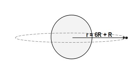
Q.A geostationary satellite is orbiting the earth at a height of 6R above the surface of earth where R is the radius of earth. The time period of another satellite at a distance of 3.5 R from the centre of earth is

(A) $16.96 hours$

(B) $8.48 hours$

(C) $9.25 hours$

(D) $15.76 hours$

Solution

We know that , orbital speed of satellite is

$v_o=\;\sqrt{\frac{GM}r}\;$

$where\;r\;is\;dis\tan ce\;from\;centre\;of\;planet/earth$

$T\;=\frac{dis\tan ce\;}{speed}=\;\frac{2\pi\;r}{v_o}$

$T\;=\;\frac{2\pi\;r}{\sqrt{\displaystyle\frac{GM}r}}$

$T\;=\;2\pi\;\sqrt{\frac{r^3}{GM}}$

$T\;=\;2\pi\;\sqrt{\frac{r^3}{GM}}\\T^2=\;4\;\pi^2\;\frac{r^3}{GM}$

$\Rightarrow T^2\;\;\propto\;r^3$

This is known as Kepler's Law of period for planetary motion

$r= R+ h$ where R is radius of planet/earth and h is height of satellite from surface of earth

$\Rightarrow r_1 = R+ 6R=7R \;and \;r_2= 3.5R$

$\Rightarrow T\;\propto\;r^\frac32$

$\frac{T_2}{T_1}=\;\left(\frac{r_2}{r_1}\right)^\frac32$

$\frac{T_2}{T_1}=\;\left(\frac{3.5R}{7R}\right)^\frac32$

$\frac{T_2}{T_1}=\;\left(\frac{1}{2}\right)^\frac32$

$\frac{T_2}{T_1}=\frac1{2\sqrt2}$

$T_2 =T_1 * \frac1{2\sqrt2}$

$T_2 =24 * \frac1{2\sqrt2}$

$T_2 =12* \frac1{\sqrt2}$

$T_2 =12* 0.707= 8.48 \;hours$

(B) is correct option

Conclusion

Kepler’s third law is also known as law of period which helps us to find the time period of orbital motion for various distances from sun. It includes following applications.

Predicting Planetary Motion: Kepler’s law of periods allows astronomers to predict the orbital periods of planets based on their distances from the sun. This law has been crucial in the study of our solar system and in the discovery and characterization of exoplanets in other solar systems.
Comparing Orbits: By comparing the orbital periods and semi-major axes of different planets or moons, astronomers can gain insights into the structure and dynamics of planetary systems. For example, comparing the orbital periods of moons around a planet can provide information about their relative distances from the planet.
Verification of Kepler’s Laws: Kepler’s laws of planetary motion played a significant role in the development of Newton’s law of universal gravitation and the laws of motion. They served as a crucial test for Newtonian physics and provided evidence for the gravitational force between celestial bodies.

Moment of Inertia of Rod having non-uniform, linearly increasing mass density

Moment of Inertia

Moment of inertia is of great importance when we come to discuss the rotational dynamics. The the word “inertia” refers to resistance against any change in state of object (mass). Specifically, the moment of inertia is measure of a body’s resistance to changes in its rotation. The greater the value of moment of inertia, the more is difficulty it is to cause change in its rotation.

The moment of inertia is often denoted as “I” and it is analogous to mass (m) of the object. In linear motion, mass quantifies an object’s resistance to linear acceleration (change in velocity) in response to a force. Similarly, in rotational motion, the moment of inertia quantifies an object’s resistance to angular acceleration (change in angular velocity) in response to a torque. Moreover, both are scalar quantities.

Factors affecting Moment of Inertia

Here are the main factors affecting the moment of inertia:

Mass Distribution
Shape of the Object
Axis of Rotation
Size and Dimensions
Symmetry

Infact, we can can generalize the above all factor into one key factor – the mass distribution of body about axis of rotation which incorporates he definition of moment of inertia.

$I= m_1 r_1^{2} + m_2 r_2^{2}+ …… m_n r_n^{2}$ . Lets consider following example to grasp the concept of moment of inertia.

Example - On Moment of Inertia of Rod

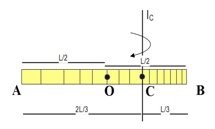
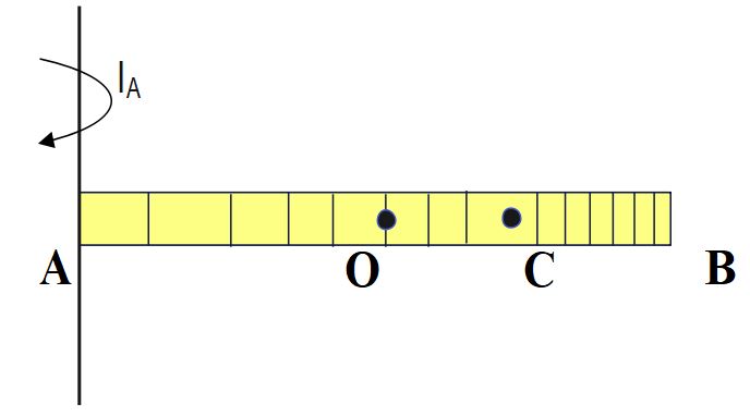
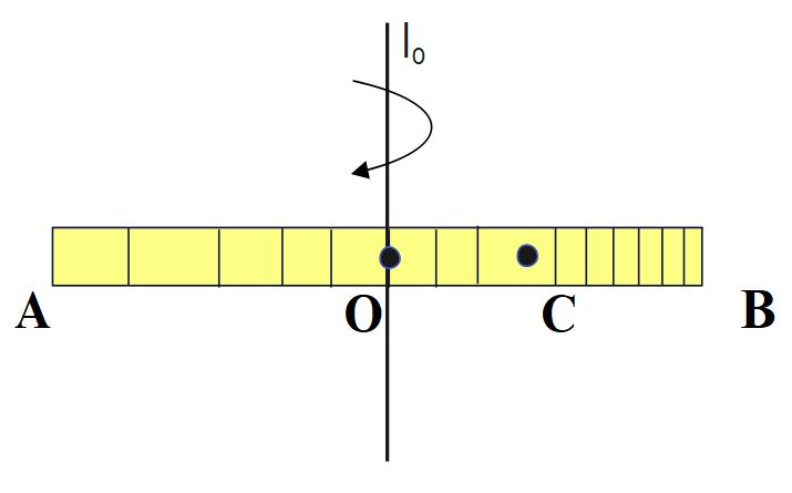
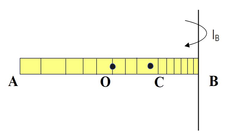
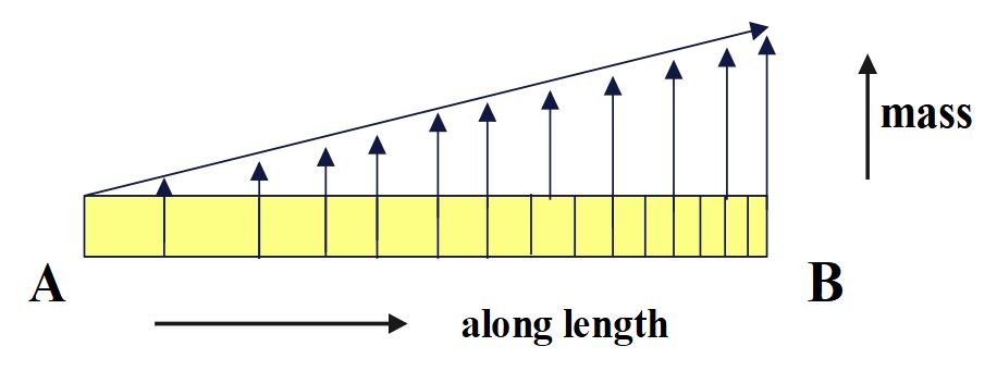
The density of a rod AB increases linearly from A to B. Its mid-point is O and centre of mass is at C. Four axes pass through A, B, O and C , all perpendicular to the length of rod. The moments of inertia of the rod about these axes are $I_{A}$ , $I_{B}$ , $I_{O}$ and $I_{C}$ respectively. Then

(A) $I_{A}> I_{B}$

(B) $I_{C}< I_{B}$

(C) $I_{O}> I_{C}$

(D) All of these

Solution

The mass distribution of body about axis of rotation determine the value of moment of inertia.

$I= m_1 r_1^{2} + m_2 r_2^{2}+ …… m_n r_n^{2}$ .

If the overall mass is distributed nearer to axis of rotation then M.O.I. of the object(rigid body) will be smaller. And if mass is distributed away from axis of rotation it results into larger M.O.I.

Let us first locate the center of mass (C.O.M.) of the rod by using formula:

x_{com}=\;\frac{\int dm\;x}{\int dm}=\frac{\int dm\;x}M

$\\x_{com}=\;\frac{\int_0^Ldm\;x}{\int_0^Ldm}=\frac{\int_0^Ldm\;x}M$ ….(1)

Given that ,the linear mass density of the rod varies linearly along the length as $\lambda\;=\lambda_o\;x$

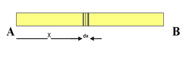
Mass of the small element dx, $dm= \lambda\ dx$

dm= \lambda_o \;x dx

By integrating on both sides, we can calculate total mass of the rod

M= \int_0^L\;dm\;=\int_0^L\;\lambda_o\;x\;dx

M=\lambda_o\;\int_0^L\;\;x\;dx

$M=\lambda_o\;\left|\frac{x^2}2\right|_0^L=\;\frac12\lambda_o\;L^2$ ….(2)

Now, we have to calculate , $\int_0^Ldm\;x\;$

\int_0^Ldm\;x\;=\;\int_0^L\;\lambda_o x\;dx\;x\;

\Rightarrow\int_0^Ldm\;x\;=\;\;\lambda_o\int_0^L\;x^2\;dx\;

\Rightarrow\;\int_0^Ldm\;x\;=\;\;\lambda_o\;\left|\frac{x^3}3\right|_0^L=\;\;\frac{\;\lambda_o\;L^3}3

$\Rightarrow\;\int_0^Ldm\;x\; =\;\;\frac{\;\lambda_o\;L^3}3$ ….(3)

From(1),(2)and (3)

x_{com}=\frac{\int_0^Ldm\;x}M\;=\frac{\frac{\;\lambda_o\;L^3}3}{\frac{\;\lambda_o\;L^2}2}\;

\Rightarrow\;x_{com}=\frac23L

According to Parallel axis theorem ,

$I_{parallel\;\;}=\;I_{COM}\;+\;M_{total\;}\;d^2$

$I_{O\;\;}=\;I_{C}\;+\;M \;(OC)^2$

$I_{B\;\;}=\;I_{C}\;+\;M \;(BC)^2$

$I_{A\;\;}=\;I_{C}\;+\;M \;(AC)^2$

AC = 2L/3 , BC = L/3, OC= L/6

As, AC > BC> OC

Hence, $I_A> I_B>I_O> I_C$

(D) is correct option

Conclusion-

In case of variable mass density total mass can be calculated by integration. And apply formula $x_{com}=\;\frac{\int dm\;x}{\int dm}$ to find position/coordinate of center of mass. Understanding of parallel axis theorem is key concept which relates all moment of inertias about any parallel axis with axis passing through centre of mass. Distribution of mass away from axis of rotation leads to greater value of moment of inertia about that axis.

Archives March 2024

Kepler's law of period